Presence detection (sparse)

An example of a presence/motion detection algorithm based on the Sparse service. Similarly to its IQ service counterpart, iq-presence-detection, this example of presence detection measures small changes in radar response over time through the difference between a fast and a slow IIR filter.

The Sparse service returns sweeps in the form of multiple subsweeps. Each subsweep constitutes of \(N_d\) range points spaced roughly 6 cm apart. We denote sweeps captured using the sparse service as \(x(f,s,d)\), where \(f\) denotes the sweep index, \(s\) the subsweep index and \(d\) the range index. As described in the documentation of the Sparse service, small movements within the field of view of the radar appear as large sinusoidal movements of the spatial sampling points over time. For each range point, we thus wish to detect any changes between individual point samples occurring in the \(s\) dimension.

In this example, this is accomplished using exponential smoothing. Two exponential filters are used, one with a larger smoothing factor, \(\alpha_{fa}\), and one with a smaller, \(\alpha_{sl}\). Each subsweep of a sweep is thus filtered through

\[x_{sl}(d) \leftarrow \alpha_{sl}x_{sl}(d) + (1 - \alpha_{sl})x(f, s, d),\]

\[x_{fa}(d) \leftarrow \alpha_{fa}x_{fa}(d) + (1 - \alpha_{fa})x(f, s, d).\]

A detection metric, \(\delta\), is obtained by taking the average difference between the two smoothed outputs as in

\[\delta = \frac{1}{N_d}\sum_{i=0}^{N_d-1}|x_{fa}(i) - x_{sl}(i)|.\]

\(\delta\) thus corresponds to amount of movement occurring in the radars field of view. Finally, \(\delta\) is thresholded to produce a prediction if movement was significant.

The presence detector can be tuned by changing the \(\alpha_{fa}\) parameter. This parameter can be related to a time constant \(\tau_{fa}\), which corresponds to what movement speeds will be detected. Increasing \(\tau_{fa}\) will also increase the noise floor in \(\delta\), so a tuning of the threshold might be necessary when altering \(\tau_{fa}\).

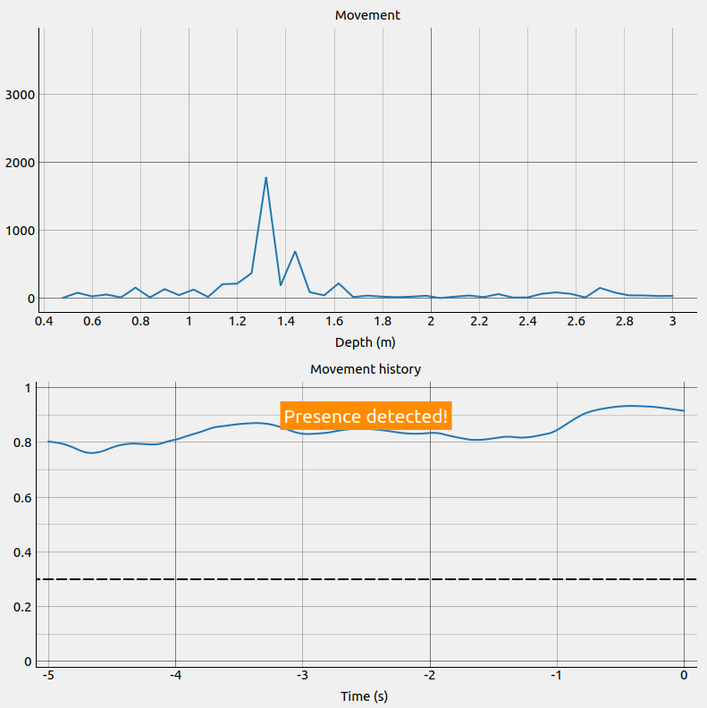
In the above image output of the sparse presence detection algorithm is shown. The top plot shows the \(|x_{fa}(d) - x_{sl}(d)|\) vector. Clear detection of a moving target is seen at a distance of roughly 1.3 m. In the bottom part the evolution of \(\delta\) is plotted. Since \(\delta\) is above the threshold of 0.3 presence is detected.

class examples.processing.presence_detection_sparse.ProcessingConfiguration

deviation_tc

Time constant of the low pass filter for the deviation between fast and slow

fast_cutoff

Cutoff frequency of the low pass filter for the fast filtered subsweep mean

noise_tc

Time constant of the low pass filter for noise estimation

output_tc

Time constant of the low pass filter for the detector output

slow_cutoff

Cutoff frequency of the low pass filter for the slow filtered subsweep mean

threshold

Level at which the detector output is considered as “present”